Using Python to Figure out Sample Sizes for your Study

It’s common wisdom among data scientists that 80% of your time is spent cleaning data, while 20% is the actual analysis.

There’s a similar issue when doing an empirical research study: typically, there’s tons of work to do up front before you get to the fun part (i.e. seeing and interpreting results).

One important up front activity in empirical research is figuring out the sample size you need. This is a crucial, since it significantly impacts the cost of your study and the reliability of your results. Collect too much sample: you’ve wasted money and time. Collect too little: your results may be useless.

Understanding the sample size you need depends on the statistical test you plan to use. If it’s a straightforward test, then finding the desired sample size can be just a matter of plugging numbers into an equation. However, it can be more involved, in which case a programming language like Python can make life easier. In this post, I’ll go through one of these more difficult cases.

Here’s the scenario: you are doing a study on a marketing effort that’s intended to increase the proportion of women entering your store (say, a change in signage). Suppose you want to know whether the change actually increased the proportion of women walking through. You’re planning on collecting the data before and after you change the signs and determine if there’s a difference. You’ll be using a two-proportion Z test for comparing the two proportions. You’re unsure how long you’ll need to collect the data to get reliable results – you first have to figure out how much sample you need!

Overview of the Two Proportion Z test

The first step in determining the required sample size is understanding the statical test you’ll be using. The two sample Z test for proportions determines whether a population proportion p1 is equal to another population proportion p2. In our example, p1 and p2 are the proportion of women entering the store before and after the marketing change (respectively), and we want to see whether there was a statistically significant increase in p2 over p1, i.e. p2 > p1.

The test test the null hypothesis: p1 – p2 = 0. The test statistic we use to test this null hypotheses is:

$latex Z = \frac{p_2 – p_1}{\sqrt{p*(1-p*)(\frac{1}{n_1} + \frac{1}{n_2})}}&s=4$

Where p* is the proportion of “successes” (i.e. women entering the store) in the two samples combined. I.e.

$latex p* = \frac{n_1p_1 + n_2p_2}{n_1 + n_2}&s=4$

Z is approximately normally distributed (i.e. ~N(0, 1)), so given a Z score for two proportions, you can look up its value against the normal distribution to see the likelihood of that value occurring by chance.

So how to figure out the sample size we need? It depends on a few factors:

  • The confidence level: How confident do we need to be to ensure the results didn’t occur by chance? For a given difference in results, detecting it with higher confidence requires more sample. Typical choices here include 95% or 99% confidence, although these are just conventions.
  • The percentage difference that we want to be able to detect: The smaller the differences you want to be able to detect, the more sample will be required.
  • The absolute values of the probabilities you want to detect differences on: This is a little trickier and somewhat unique to the particular test we’re working with. It turns out that, for example, detecting a difference between 50% and 51% requires a different sample size than detecting a difference between 80% and 81%. In other words, the sample size required is a function of p1, not just p1 – p2.
  • The distribution of the data results: Say that you want to compare proportions within sub-groups (in our case, say you subdivide proportion of women by age group). This means that you need the sample to be big enough within each subgroup to get statistically significant comparisons. You often don’t know how the sample will pan out within each of these groups (it may be much harder to get sample for some). There are at least a couple of alternatives for you here: i) you could assume sample is distributed uniformly across subgroups ii) you can run a preliminary test (e.g. sit outside the store for half a day to get preliminary proportions of women entering for each age group).

So, how do you figure out sample sizes when there are so many factors at play? 

Figuring out Possibilities for Sample Sizes with Python

Ultimately, we want to make sure we’re able to calculate a difference between p1 and p2 when it exists. So, let’s assume you know that the “true” difference that exists between p1 and p2. Then, we can look at sample size requirements for various confidence levels and absolute levels of p1.

We need a way of figuring out Z, so we can determine whether a given sample size provides statistically significant results, so let’s define a function that returns the Z value given p1, p2, n1, and n2.

[gist https://gist.github.com/marknagelberg/b6bfe3e2141f8eeaeb0f2537ccbed81f /]

Then, we can define a function that returns the sample required, given p1 (the before probability), pdiff (i.e. p2 – p1), and alpha (which represents the p-value, or 1 minus the confidence level). For simplicity we’ll just assume that n1 = n2. If you know in advance that n1 will have about a quarter of the size of n2, then it’s trivial to incorporate this into the function. However, you typically don’t know this in advance and in our scenario an equal sample assumption seems reasonable.

The function is fairly simplistic: it counts up from n starting from 1, until n gets large enough where the probability of that statistic being that large (i.e. the p-value) is less than alpha (in this case, we would reject the null hypothesis that p1 = p2). The function uses the normal distribution available from the scipy library to calculate the p value and compare it to alpha. 

[gist https://gist.github.com/marknagelberg/42b3077db573bcce55e00f975b8e4fc5 /]

These functions we’ve defined provide the main tools we need to determine minimum sample levels required.

As mentioned earlier, one complication to deal with is the fact that the sample required to determine differences between p1 and p2 depend on the absolute level of p1. So, the first question we want to answer is “what p1 that would require the biggest sample size to determine a given difference with p2?” Figuring this out allows you to calculate a lower bound on the sample you need for any p1. If you calculate the sample for the p1 with the highest required sample, you know it’ll be enough for any other p1.

Let’s say we want to be able to calculate a 5% difference with 95% confidence level, and we need to find a p1 that gives us the largest sample required. We first generate a list in Python of all the p1 to look at, from 0% to 95% and then use the sample_required function for each difference to calculate the sample.

[gist https://gist.github.com/marknagelberg/6b0679187cd7ce110546e581417bf6c4 /]

Then, we plot the data with the following code.

[gist https://gist.github.com/marknagelberg/2ace5e06f7012c76936887d82eff6aaf /]

Which produces this plot:

This plot makes it clear that p1 = 50% produces the highest sample sizes.

Using this information, let’s say we want to calculate the sample sizes required to calculate differences in p1 and p2 where p2 – p1 is between  2% and 10%, and confidence levels are 95% or 99%. To ensure we get a sample large enough, we know to set p1 = 50%. We first write the code to build up the data frame to plot.

[gist https://gist.github.com/marknagelberg/4e647533f034a244ea3850e6ab5ec4da /]

Then we write the following code to plot the data with Seaborn.

[gist https://gist.github.com/marknagelberg/0c1845bf835da661851c948d837a0e95 /]

The final result is this plot:

This shows the minimum sample required to detect probability differences between 2% and 10%, for both 95% and 99% confidence levels. So, for example, detecting a difference of 2% at 95% confidence level requires a sample of ~3,500, which translates into n1 = n2 = 1,750. So, in our example, you would need about 1,750 people walking into the store before the marketing intervention, and 1,750 people after to detect a 2% difference in probabilities at a 95% confidence level.

Conclusion

The example shows how Python can be a very useful tool for performing “back of the envelope” calculations, such as estimates of required sample sizes for tests where this determination is not straightforward. These calculations can save you a lot of time and money, especially when you’re thinking about collecting your own data for a research project.
How to Find Underrated People on Twitter with TURI (Twitter Underrated Index)

One of the best skills that you can develop is the ability to find talented people before anyone else does.

This great advice from Tyler Cowen (economist and blogger at Marginal Revolution) got me thinking: What are some strategies for finding talented but underrated people?

One possible source is Twitter. For a long time, I didn’t “get” Twitter, but after following Michael Nielsen’s advice I’m officially a convert. The key is carefully selecting the list of people you follow. If you do this well, your Twitter feed becomes a constant stream of valuable information and interesting people.

If you look carefully, you can find a lot of highly underrated people on Twitter, i.e. incredibly smart people that put out valuable and interesting content, but have a smaller following that you would expect.

These are the kinds of people that are the best to follow: you get access to insights that a lot of other people are not getting (since not many people are following them), and they are more likely to respond to queries or engage in discussion (since they have a smaller following to manage).

One option for finding these people is trial and error, but I wanted to see if it’s possible to quantify how underrated people are on Twitter and automate the process for finding good people to follow.

I call this the TURI (Twitter Underrated Index), because hey, it needs a name and acronyms make things sound so official.

Components of TURI

The index has three main components: Growth, Influence of Followers, and the Number of Followers.

Growth (G): The number of followers a user has per unit of content they have published (i.e. per tweet).

A user that is growing their Twitter following quickly suggests that they are underrated. It implies they are putting out quality content and people are starting to notice rapidly. The way I measure this is the number of followers a person acquires per Tweet.

Another possible measurement of growth is the number of followers the user has acquired per unit of time (i.e. number of followers divided by the length of time the Twitter account has existed). However, there are a couple of problems with this option:

  • Twitter accounts can be dormant for years. For example, someone might start an account but not tweet for 5 years and then put out great content. Measuring growth in terms of time would unfairly punish these people.
  • A person may have a strategy of Tweeting constantly. Some of the content results in followers, but the overall quality is still low. We are looking for people that publish great content, not necessarily people that put out a lot of content.

Influence of Followers (IF): The average number of the user’s follower’s followers.

In my opinion, the influence of a person’s following is the most important factor determining whether they are underrated on Twitter. Here’s a few reasons why:

  • Influential people are, on average, better judges of good content.
  • Influential people are more selective in who they decide to follow, especially if Twitter is an important part of their online “brand”.
  • Influential people tend to engage with or are in some way related to other high quality people in their offline personal lives, and these people are more likely to appear in their Twitter feed even if they are not widely known or appreciated yet.

I’m somewhat biased toward this measure because, from my own personal experience, it has worked out really well when I browse through people who are followed by influential people on my feed. If I see someone followed by Tyler Cowen, Alex Tabarrok, Russ Roberts, Patrick Collison, and Marc Andreessen, and yet they only have 5,000 followers, then I’m pretty confident that person is currently underrated.

After some consideration, I believe the best way to measure the influence of a user’s followers with the data available in the Twitter API is taking the average number of the user’s follower’s followers.

I mulled over the possibility of using the median rather than the average, but decided against it: If someone with 1 million followers follows someone with 50 followers, I want to know more about that person, even though their TURI is high only because of that one highly influential follower. Outliers are good – we’re looking for diamonds in the rough.

Total Number of Followers (NF): The total number of followers the user currently has.

Our very definition of “underrated” in this context is when a user does not have as many followers as you expect, so total number of followers is obviously going to play an important role in TURI.

So to summarize the main idea behind TURI: if a person has a large number of “influential” followers, is growing their number of followers quickly relative to the volume of content they put out, and they still have a small number of total followers, then they are likely underrated.

Defining the Index

For any user i, we can calculate their Twitter Underrated Index (TURI) as:

$latex TURI_i = \frac{G_iIF_i}{NF_i}&s=4$

Where G is growth, IF is influence of followers, and NF is the number of followers.

This formula has the general relationships we are looking for: high growth in users for each unit of content, highly influential followers, and a low number of total followers all push TURI upward.

We can simplify the equation by rewriting G = NF / T, where T is the total number of tweets for the user. Cancelling out some terms, this gives us our final version of the index:

$latex TURI_i = \frac{IF_i}{T_i}&s=4$

In other words, our index of how under-rated a person is on twitter is given by the average number of i’s followers followers per tweet of user i.

Before calculating TURI for a group of users, there are a couple of pre-processing steps you will likely want to take to improve the results:

  1. Filter out verified accounts. One of the shortcomings of TURI is that a user’s growth / trajectory (i.e. G) will be very high if they are already a celebrity. These people typically have a large number of followers per Tweet not because of the content they put out, but because they’ve attained fame already elsewhere. Luckily, Twitter has a feature called a “verified account”, which applies “if it is determined to be an account of public interest. Typically this includes accounts maintained by users in music, acting, fashion, government, politics, religion, journalism, media, sports, business, and other key interest areas”. This is a prime group to filter out, because we are not looking for well-known people.
  2. Filter users by number of followers: There are a few reasons why you might want to only calculate TURI for users that have a following within some range (e.g. between 500 and 1,000):
    • Although there may be situations where a person with 500,000 followers is underrated, but this seems unlikely to be the kind of person you’re looking for so not worth the API resources.  
    • Filtering by some upper follower threshold mitigates the risk of including celebrities without verified accounts.
    • You limit the number of calls you make to the API. The most costly operation in terms of API calls is figuring out the influence of followers. The more followers a person has, the more API calls required to calculate TURI.

Trying out TURI

To test out the index, I calculated its value on a subset of 49 people that Tyler Cowen follows who have 1,000 or fewer followers (Tyler blogs at my favourite blog, inspired this project, and has good taste in people to follow).

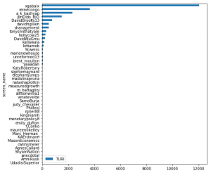
The graph below illustrates TURI for these users (not including 4 accounts that were not accessible due to privacy settings). 

As you can see, one user (@xgabaix) is a significant outlier. Looking a bit more closely at the profile, this is Xavier Gabaix, a well known economist at Harvard University. His TURI is so high because he has several very influential followers and he has not tweeted yet. 

So did TURI fail here? I don’t think so, since this is very likely someone to follow if he was actually Tweeting. However, it does seem a little strange to put someone at the top of the list that doesn’t actually have any Twitter content.

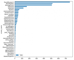
So, I filtered again for users that have published at least 20 tweets:

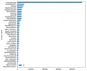
The following chart looks solely at the various user’s IF (Influence of their Followers). Interestingly, another user @shanagement has the most influential followers by far. However, they rank in third place for overall TURI since they tweet significantly more than @davidbrooks13 or @davidhgillen.

Limitations

Of course, TURI has some shortcomings:

  • Difficult to tell how well TURI works: The measures are based on intuition and there is obviously no “ground truth” data about how underrated twitter users actually are. So, we don’t really have a data-based method for seeing how well the index works and improving it systematically. For example, you might question is whether Growth G should be included in the index at all. I think there’s a good argument for it: if people get followers quickly per unit of content there must be something about that content that draws others. But, on the other hand, maybe they aren’t truly underrated. Maybe the truly underrated people have good content but your average Twitter user underestimates them even after reading a few posts. People don’t always know high quality when the see it.
  • It takes a fairly long time to calculate TURI: This is due to Twitter rate limits of API requests. For example, calculating TURI for 49 Twitter users above took about an hour. It would take even longer for people with larger followings (remember, I only focused on people with 1,000 or fewer followers). So, if you want to do a large batch of people, it’s probably a good idea run this on a server on an ongoing basis and store user and TURI information into a database. 

Other ideas?

There are many many different ways you could potentially specify an index like this. Leave a comment or reach out to me on Twitter or email if you have any suggestions.

One other possible tweak is accounting for the number of people that the user follows. I notice that some Twitter users seem to have a strategy of following a huge number of people in the hopes of being followed back. In these cases, their following strategy may be the cause of their high growth and not the quality of their content. One solution is to adjust the TURI by multiplying by (Number of User’s Followers) / (Number of People the User Follows). This would penalize people that, for example, have 15,000 followers but follow 15,000 people themselves.

Technical Details

You can find the code I used to interact with the API and calculate TURI here. The code uses the python-twitter package, which provides a nice way of interacting with the Twitter API, abstracting away annoying details so you don’t have to deal with them (e.g. authenticating with OAuth, dealing with rate limits).