- Author:: [[Ralph Kimball]], [[Margy Ross]]
- Reading Status:: #complete
- Review Status:: #[[complete]]
- Tags:: #books #[[dimensional modeling]]
- Source:: link
- Roam Notes URL:: link
- Anki Tag:: kimball_group_reader kimball_group_reader_ch_1
- Anki Deck Link:: link
- Setting up for Success
- 1.1 Resist the Urge to Start Coding ([[Ralph Kimball]], DM Review, November 2007) (Location 944)
- Before writing any code or doing any modelling or purchasing related to your data warehouse, make sure you have a good answer to the following 10 questions:
- [[Business Requirements]]: do you understand them? (Most fundamental and far-reaching question)
- [[Strategic Data Profiling]]: are data assets available to support business requirements?
- [[Tactical Data Profiling]]: Is there executive buy-in to support business process changes to improve data quality?
- [[Integration]]: Is there executive buy-in and communication to define common descriptors and measures?
- [[Latency]]: Do you know how quickly data must be published by the data warehouse?
- [[Compliance]]: which data is compliance-sensitive, and where must you have protected chain of custody?
- [[Data Security]]: How will you protect confidential or proprietary data?
- [[Archiving Data]]: How will you do long-term archiving of important data and which data must be archived?
- [[Business User Support]]: Do you know who the business users are, their requirements and skill level?
- [[IT Support]]: Can you rely on existing licenses in your organization, and do IT staff have skills to support your technical decisions?
- Before writing any code or doing any modelling or purchasing related to your data warehouse, make sure you have a good answer to the following 10 questions:
- 1.2 Set Your Boundaries ([[Ralph Kimball]], DM Review, December 2007) (Location 1003) #[[Business Requirements]] #[[setting boundaries]]
- This article is a discussion of setting clear boundaries in your data warehousing project to avoid taking on too many requirements.
- 1.1 Resist the Urge to Start Coding ([[Ralph Kimball]], DM Review, November 2007) (Location 944)
- Tackling DW/BI Design and Development
- This group of articles focuses on the big issues that are part of every DW/BI system design. (Location 1071)
- 1.3 Data Wrangling ([[Ralph Kimball]], DM Review, January 2008) (Location 1074) #[[data wrangling]] #[[data extraction]] #[[data staging]] #[[change data capture]]
- [[data wrangling]] is the first stage of the data pipeline from operational sources to final BI user interfaces in a data warehouse. It includes [[change data capture]], [[data extraction]], [[data staging]], and [[data archiving]] (Location 1076)
- [[change data capture]] is the process of figuring out exactly what data changed on the source system that you need to extract. Ideally this step would be done on source production system. (Location 1080). Two approaches:
- Using a change_date_time field in the source: a good option, but will miss record deletion and any override of the trigger producing the change_date_time field. (Location 1089)
- Production system daemon capturing every input command: This detects data deletion but there are still DBA overrides to worry about. (Location 1089)
- Ideally you will also get your source production system to provide a reason data changed, which tells you how the attribute should be treated as a [[slowly changing dimension (SCD)]]. (Location 1098) #[[change data capture]]
- If you can’t do [[change data capture]] on source production system, you’ll have to do it after extraction, which means downloading larger data sets. (Location 1103)
- Consider using [[cyclic redundancy checksum (CRC)]] to significant improve performance of the data comparison step here.
- [[data extraction]]: The transfer of data from the source system into the DW/BI environment. (Location 1117)
- Two main goals in the [[data extraction]] step:
- Remove proprietary data formats
- Move data into [[flat files]] or [[relational tables]] (eventually everything loaded into relational tables, but flat tiles can be processed very quickly)
- Two main goals in the [[data extraction]] step:
- [[data staging]]: [[Ralph Kimball]] recommends staging ALL data: save the data the DW/BI system just received in original target format you chose before doing anything else to it. (Location 1126)
- [[data archiving]]: this is important for compliance-sensitive data where you have to prove data received hasn’t been tampered with. Techniques here include using a [[hash code]] to show data hasn’t changed. (Location 1129)
- 1.4 Myth Busters ([[Ralph Kimball]], DM Review, February 2008) (Location 1135) #[[dimensional modeling]]
- Addresses various myths related to [[dimensional modeling]]
- Myth: A dimensional model could be missing key relationships that exist only in a true relational view. (Location 1142)
- In fact, dimensional models contain all the data relationships that normalized models have.
- Myth: dimensional models are not sufficiently extensible and do not accommodate changing [[business requirements]]. (Location 1149)
- It’s the opposite: normalized models are much harder to change when data relationships change. [[slowly changing dimension (SCD)]] techniques provide the basis for models to meet changing [[business requirements]].
- Myth: dimensional models don’t capture data at sufficient level of granularity / detail (Location 1177)
- In fact, models should capture measurement events in [[fact tables]] at the lowest possible grain.
- 1.5 Dividing the World ([[Ralph Kimball]], DM Review, March 2008) (Location 1188)
- Two main entities in [[dimensional modeling]] (Kimball estimates 98% of data can be immediately and obviously categorized as one of these):
- [[dimension ([[dimensional modeling]])]]: the basic stable entities in our environment, such as customers, products, locations, marketing promotions, and calendars. In end user BI tools, dimensions are primarily used for constraints and row headers.
- [[fact ([[dimensional modeling]])]]: Numeric measurements or observations gathered by all of our transaction processing systems and other systems. In end user BI tools, dimensions are primarily used for computations.
- [[fact table grain]]: Description of measurement in physical, real-world terms – a description of what each row in the [[fact table]] represents. (Location 1209) There is sometimes a temptation to add facts not true to the grain to shortcut a query, but this often introduces complexity and confusion for business users. (Location 1218)
- A [[fact ([[dimensional modeling]])]] should be additive whenever possible – it should make sense to add facts across records. A common example here is storing extended price (i.e. price * quantity) instead of just price in a fact table where the measurement is retail sale (Location 1224)
- A distinct characteristic of [[dimensional modeling]] is not using [[normalized data]]. Normalized models are great in transaction processing systems, but they are not understandable by business users. Dimensional models, correctly designed, contain exactly the same data and reflect the same business rules, but are more understandable. [[understandability]] is a central goal of a BI system used by business users. (Location 1249)
- Two main entities in [[dimensional modeling]] (Kimball estimates 98% of data can be immediately and obviously categorized as one of these):
- 1.6 Essential Steps for the Integrated [[Enterprise Data Warehouse (EDW)]] ([[Ralph Kimball]], DM Review, April 2008 and May 2008) (Location 1254) #[[data integration]]
- This section provides an overall architecture for building an integrated [[Enterprise Data Warehouse (EDW)]] which supports [[Master Data Management (MDM)]] and and has the mission of providing a consistent business analysis platform for an organization. (Location 1258)
- Essential act of the [[Enterprise Data Warehouse (EDW)]] is [[drilling across]]: gathering results from separate [[business process subject area]]s and combine them into a single analysis. (Location 1282)
- A key prerequisite to developing the [[Enterprise Data Warehouse (EDW)]] is a significant commitment and support from top-level mangement on the value of data integration. (Location 1303)
- Having an existing [[Master Data Management (MDM)]] project is a good sign of executive buy-in for data integration, and significantly simplifies data warehouse [[data integration]]. (Location 1308)
- [[conformed dimensions]] and [[confirmed facts]] provide the basis for [[data integration]] (Location 1316)
- [[conformed dimensions]]: two dimensions are conformed if they contain one or more common fields whose contents are drawn from the same domains. (Location 1318) Typical examples: customer, product, service, location, employee, promotion, vendor, and calendar. (Location 1367)
- [[conformed facts]]: numeric measures that have the same business and mathematical interpretations so that they may be compared and computed against each other consistently. (Location 1320)
- [[enterprise data warehouse (EDW) bus matrix]]: two-dimensional matrix with [[business process subject area]] on the vertical axis and [[dimension tables]] on horizontal axis. (Location 1324) An X in the matrix represents where a subject area uses a dimension. It helps you prioritize development of separate subject areas and identify possible scope of [[conformed dimensions]]. "The columns of the bus matrix are the invitation list to the conformed dimension design meeting." (Location 1333) This is an important item to send to senior management to review before conformed dimension design meetings. "If senior management is not interested in what the bus matrix implies, then to make a long story short, you have no hope of building an integrated EDW." (Location 1335)
- Note that the different stakeholders don’t have to give up their domain specific private attributes that they need – stakeholders just need to agree on the [[conformed dimensions]]. (Location 1341)
- Even when you get senior management full buy-in, there is a lot of operational management involved in the [[Enterprise Data Warehouse (EDW)]], including two abstract figures: the [[dimension manager]] (builds and distributes a conformed dimension to the rest of the enterprise) and the [[fact provider]] (downstream client to the dimension manager who receives and utilizes the conformed dimension, almost always while managing one or more fact tables within a subject area). (Location 1347)
- 1.7 Drill Down to Ask Why [[Ralph Kimball]], DM Review, July 2008 and August 2008 (Location 1481) #[[decision making]]
- Important to understand how your data warehousing system drives decision-making, not just your technical architecture.
- [[Bill Schmarzo]] architecture for decision making, aka [[analytic application process]]: (Location 1489)
- Publish reports.
- Identify exceptions.
- Determine causal factors. Seek to understand the “why” or root causes behind the identified exceptions. Main ways you might do this: #[[causality]] #[[determining causality]]
- Get more detail
- Get a comparison
- Search other data sets
- Search the web for information about the problem
- Model alternatives. Provide a backdrop to evaluate different decision alternatives.
- Track actions. Evaluate the effectiveness of the recommended actions and feed the decisions back to both the operational systems and DW, against which published reporting will occur, thereby closing the loop.
- 1.8 Slowly Changing Dimensions [[Ralph Kimball]], DM Review, September 2008 and October 2008 (Location 1557) #[[slowly changing dimension (SCD)]]
- The Original Three Types of [[slowly changing dimension (SCD)]] cover all the responses required for a revised or updated description of a dimension member (Location 1569)
- [[type 1 slowly changing dimension (SCD)]]: Overwrite
- [[type 2 slowly changing dimension (SCD)]]: Add a New Dimension Record
- [[type 3 slowly changing dimension (SCD)]]: Add a New Field
- The Original Three Types of [[slowly changing dimension (SCD)]] cover all the responses required for a revised or updated description of a dimension member (Location 1569)
- 1.9 Judge Your BI Tool through Your Dimensions – [[Ralph Kimball]], DM Review, November 2008 (Location 1650) #[[BI tools]] #[[BI tool selection]] #[[dimension tables]]
- [[dimension tables]] implement the [[UI]] of your BI system: they provide the labels, the groupings, the drill-down paths.
- This article describes [[requirements]] a BI tool should be able to meet with dimensions:
- Assemble a BI query or report request by first selecting [[dimension table attributes]] and then selecting [[facts (dimensional modelling)]] to be summarized.
- [[drilling down]] by adding a row header
- Browse a dimension to preview permissible values and set constraints
- Restrict the results of a dimension browse with other constraints in effect
- [[drilling across]] by accumulating measures under labels defined by conformed dimension attributes
- 1.10 [[fact tables]] – [[Ralph Kimball]], DM Review, December 2008 (Location 1707)
- [[fact tables]] contain the fundamental measurements of the enterprise and are the target of most data warehouse queries.
- Design rules for [[fact tables]]:
- Stay true to the [[fact table grain]] – take care in defining the [[grain (dimensional modelling)]] – what a single record in the fact table represents. This is the first and most important design step. It ensures the [[foreign keys]] in the fact table are grounded and precise.
- Build up from the lowest possible [[fact table grain]]. This ensures you have the most complete set of [[dimension tables]] that can describe the fact table and enables detailed [[drilling down]] for the user.
- 3 types of [[fact tables]]: (Location 1741)
- [[transaction grain [[fact table]]]]: Measurement taken at a single instance (e.g. each cash register beep). Transactions can happen after a millisecond or next month or never – they’re unpredictably sparse or dense.
- [[periodic snapshot grain [[fact table]]]]: Facts cover a predefined span of time. Powerful guarantee: all reporting entities will appear in each snapshot, even if there is no activity – it’s predictably dense and applications can rely on certain key combinations being available.
- [[accumulating snapshot grain [[fact table]]]]: Rows represent a predictable process with a well-defined beginning and end (e.g. order processing, claims processing).
- 1.11 Exploit Your [[fact tables]] – [[Ralph Kimball]], DM Review, January/February 2009 (Location 1765)
- This article describes basic ways to exploit the 3 main fact table designs in the front room and in the back room.
- Front Room: [[aggregate navigation]] – choosing to give the user pre-aggregated data at run time, without without the end user knowing the difference. Seamlessly provide aggregated and detailed atomic data.
- Front Room: [[drilling across]] Multiple Fact Tables at Different Grains – you can do this as long as you choose [[conformed dimensions]] for the answer set row headers that exist for all the fact tables in your integrated query.
- Front Room: Exporting Constraints to Different Business Processes – building connections to other [[business process subject area]] in the [[UI]] so you can explore related data in a single click or swipe.
- Back Room: [[fact table surrogate keys (FSKs)]] – sometimes you want to do this for one of the following benefits
- Uniquely and immediately identify single fact records.
- FSKs assigned sequentially so a load job inserting new records will have FSKs in a contiguous range.
- An FSK allows updates to be replaced by insert-deletes.
- An FSK can become a foreign key in a fact table at a lower grain.
Tag: data engineering
Getting Started with Airflow Using Docker
Lately I’ve been reading intensively on data engineering after being inspired by this great article by Robert Chang providing an introduction to the field. The underlying message of the article really resonated with me: when most people think of data science they immediately think about the stuff being done by very mature tech companies like Google or Twitter, like deploying uber-sophisticated machine learning models all the time.
However, many organizations are not at the stage where these kind of models makes sense as a top priority. This is because, to build and deploy these kind of models efficiently and effectively, you need to have foundation data infrastructure in place that you can build the models on. Yes, you can develop a machine learning model with the data you have in your organization, but you have to ask: how long did it take you to do it, is your work repeatable / automatable, and are you able to deploy or actually use your solution in a meaningful and reliable way? This is where data engineering comes in: it’s all about building the data warehouses and ETL pipelines (extract-transform-load) that provide the fundamental plumbing required to do everything else.
One tool that keeps coming up in my research on data engineering is Apache Airflow, which is “a platform to programmatically author, schedule and monitor workflows”. Essentially, Airflow is cron on steroids: it allows you to schedule tasks to run, run them in a particular order, and monitor / manage all of your tasks. It’s becoming very popular among data engineers / data scientists as a great tool for orchestrating ETL pipelines and monitor them as they run.
In this post, I’ll give a really brief overview of some key concepts in Airflow and then show a step-by-step deployment of Airflow in a Docker container.
Key Airflow Concepts
Before we get into deploying Airflow, there are a few basic concepts to introduce. See this page in the Airflow docs which go through these in greater detail and describe additional concepts as well.
Directed Acyclic Graph (DAG): A DAG is a collection of the tasks you want to run, along with the relationships and dependencies between the tasks. DAGs can be expressed visually as a graph with nodes and edges, where the nodes represent tasks and the edges represent dependencies between tasks (i.e. the order in which the tasks must run). Essentially, DAGs represent the workflow that you want to orchestrate and monitor in Airflow. They are “acyclic”, which means that the graph has no cycles – in English, this means means your workflows must have a beginning and an end (if there was a cycle, the workflow would be stuck in an infinite loop).
Operators: Operators represent what is actually done in the tasks that compose a DAG workflow. Specifically, an operator represents a single task in a DAG. Airflow provides a lot of pre-defined classes with tons of flexibility about what you can run as tasks. This includes classes for very common tasks, like BashOperator, PythonOperator, EmailOperator, OracleOperator, etc. On top of the multitude of operator classes available, Airflow provides the ability to define your own operators. As a result, a task in your DAG can do almost anything you want, and you can schedule and monitor it using Airflow.
Tasks: A running instance of an operator. During the instantiation, you can define specific parameters associated with the operator and the parameterized task becomes a node in a DAG.
Deploying Airflow with Docker and Running your First DAG
This rest of this post focuses on deploying Airflow with docker and it assumes you are somewhat familiar with Docker or you have read my previous article on getting started with Docker.
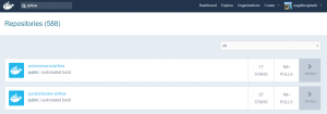
As a first step, you obviously need to have Docker installed and have a Docker Hub account. Once you do that, go to Docker Hub and search “Airflow” in the list of repositories, which produces a bunch of results. We’ll be using the second one: puckel/docker-airflow which has over 1 million pulls and almost 100 stars. You can find the documentation for this repo here. You can find the github repo associated with this container here.
So, all you have to do to get this pre-made container running Apache Airflow is type:
docker pull puckel/docker-airflow
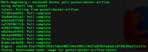
And after a few short moments, you have a Docker image installed for running Airflow in a Docker container. You can see your image was downloaded by typing:
docker images
![]()
Now that you have the image downloaded, you can create a running container with the following command:
docker run -d -p 8080:8080 puckel/docker-airflow webserver
Once you do that, Airflow is running on your machine, and you can visit the UI by visiting http://localhost:8080/admin/
On the command line, you can find the container name by running:
docker ps
You can jump into your running container’s command line using the command:
docker exec -ti <container name> bash
So in my case, my container was automatically named competent_vaughan by docker, so I ran the following to get into my container’s command line:
![]()
Running a DAG
So your container is up and running. Now, how do we start defining DAGs?
In Airflow, DAGs definition files are python scripts (“configuration as code” is one of the advantages of Airflow). You create a DAG by defining the script and simply adding it to a folder ‘dags’ within the $AIRFLOW_HOME directory. In our case, the directory we need to add DAGs to in the container is:
/usr/local/airflow/dags
The thing is, you don’t want to jump into your container and add the DAG definition files directly in there. One reason is that the minimal version of Linux installed in the container doesn’t even have a text editor. But a more important reason is that jumping in containers and editing them is considered bad practice and “hacky” in Docker, because you can no longer build the image your container runs on from your Dockerfile.
Instead, one solution is to use “volumes”, which allow you to share a directory between your local machine with the Docker container. Anything you add to your local container will be added to the directory you connect it with in Docker. In our case, we’ll create a volume that maps the directory on our local machine where we’ll hold DAG definitions, and the locations where Airflow reads them on the container with the following command:
docker run -d -p 8080:8080 -v /path/to/dags/on/your/local/machine/:/usr/local/airflow/dags puckel/docker-airflow webserver
The DAG we’ll add can be found in this repo created by Manasi Dalvi. The DAG is called Helloworld and you can find the DAG definition file here. (Also see this YouTube video where she provides an introduction to Airflow and shows this DAG in action.)
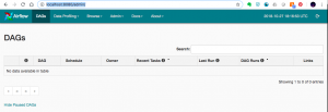
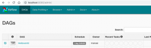
To add it to Airflow, copy Helloworld.py to /path/to/dags/on/your/local/machine. After waiting a couple of minutes, refreshed your Airflow GUI and voila, you should see the new DAG Helloworld:
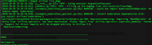
You can test individual tasks in your DAG by entering into the container and running the command airflow test. First, you enter into your container using the docker exec command described earlier. Once you’re in, you can see all of your dags by running airflow list_dags. Below you can see the result, and our Helloworld DAG is at the top of the list:
One useful command you can run on the command line before you run your full DAG is the airflow test command, which allows you to test individual tests as part of your DAG and logs the output to the command line. You specify a date / time and it simulates the run at that time. The command doesn’t bother with dependencies and doesn’t communicate state (running, success, failed, …) to the database, so you won’t see the results of the test in the Airflow GUI. So, with our Helloworld DAG, you could run a test on task_1
airflow test Helloworld task_1 2015-06-01
Note that when I do this, it appears to run without error; however, I’m not getting any logs output to the console. If anyone has any suggestions about why this may be the case, let me know.
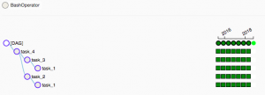
You can run the backfill command, specifying a start date and an end date to run the Helloworld DAG for those dates. In the example below, I run the dag 7 times, each day from June 1 – June 7, 2015:
![]()
When you run this, you can see the following in the Airflow GUI, which shows the success of the individual tasks and each of the runs of the DAG.
Resources
- I was confused about whether you can create DAGs with the UI, and this Stackoverflow Thread seems to indicate that you can’t. Note in the answer the responder mentions a few potentially useful tools for developing a UI where users can define DAGs without knowing Python.
- This Stackoverflow thread was helpful for figuring out that volumes are the solution to add DAGs to Airflow running in a container.
- Official tutorial from Apache Airflow
- Common Pitfalls Associated with Apache Airflow
- ETL Best Practices with Airflow