Category: Articles

Testing is an important part of development, including developing web applications. Among other benefits, they increase your confidence that your web application is doing what you expect, and a provide a basis for preventing bugs in an automated way when you make changes to your code.

Since testing is such an integral part of web application maintenance and deployment, in this Part 3 of our app-deploy project we’ll put in some basic tests to see how they can be implemented in flask applications and so we will eventually see how tests fit into the deployment workflow. We’ll be using the pytest python library as our testing framework.

To follow along, you can clone the repository:

git clone https://github.com/marknagelberg/app-deploy.git

And then go to the appropriate location in the code with the following command which includes all of the changes made in this post:

git checkout ed2ed02f8b3db

Finally, create the python environment with:

conda env create -f environment.yml

First, a Slight Upgrade to our App

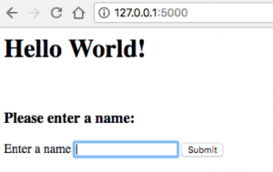
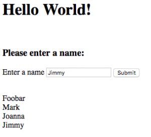
Right now, when out user enters information into the app’s simple web form, the data is simply added to the database and nothing changes from the user’s perspective. To make testing a bit more interesting, we first add a little bit of additional functionality: our app will now print out a list of all the existing names in the database on the main page.

First we add a few lines to app/app.py so that it queries the database to get all names, and then sends the list of names to the template.

https://gist.github.com/marknagelberg/f4cb543ca596d383362ef9383b03ee6a

Then, we update the template to print out these names.

https://gist.github.com/marknagelberg/5b2237cc9157bdbe84b9b3283d0ba133

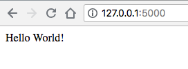
Now, when you enter in new names, they are listed out for you, like so:

Pytest Installation and Set-up

To start off, let’s activate our app’s conda environment and install pytest:

source activate app-deploy
conda install pytest

Our tests will be stored in a top level directory in a folder that we’ll call `tests`. Our tests will be stored in *.py files within this folder. These files must either be named like test_*.py or *_test.py: this is how you tell pytest that these files represent tests (in other words, this is how pytest does “test discovery”).

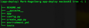
As a reminder, your top level directory should look something like this:

So, let’s add a file called test_app.py in /test.

touch test/test_app.py

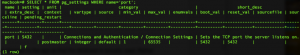
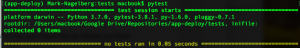
To run your tests, you simply just have to enter ‘pytest’ in the command line as follows. No tests have been added to test_app.py yet, so when you run ‘pytest’ now, the result should look like this:

A couple of other small preliminaries to get testing set up:

• Set WTF_CSRF_ENABLED configuration variable equal to False in the testing configuration found in config.py. This is required for tests to run properly. Keep in mind that you normally want to have this set equal to True when you’re running your application in production, since this protects your forms against Cross Site Request Forgery (CSRF) attacks.
• Add __init__.py in your /tests directory.

Adding Tests

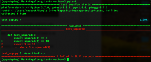
The great thing about pytest is that it allows you to write tests in a very concise, pythonic way using assert statements. Suppose you have the following file which defines a function that takes the square of a number. You want to test this. Adding a couple of tests is as easy as this:

https://gist.github.com/marknagelberg/aa99d1be3dca7149c12f0be984a0542a

Then, you run your tests by typing `pytest` in the command line when you’re in the app’s main directory. This returns the following result (one test pass, one test fail):

Another great feature of pytest is the ability to produce “fixtures”, which provides tests with pre-initialized objects you require to run your tests. In our case, a great use of fixtures is initializing the test database or the test application instance.

Pytest fixtures have some advantages over the usual setup and teardown functions used in other testing frameworks. One is the ability to run fixtures using different “scopes”, allowing you to do the setup / teardown operation at different times when you run your test to maximize test efficiency. The options for scope here include function, class, module, and session. So, for example, a fixture in the function scope means that the fixture object is invoked once for each test function you define in pytest.

So, say all your tests need to be able to access the Flask test client application instance. Using the module fixture, the application instance is only created once at the very beginning when you run your test, rather than being created and destroyed once for every test function.

For our small app, we’ll create 3 fixtures:

• A database record in our Name table
• The Flask application instance
• The test database

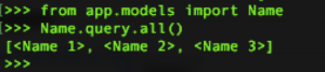
The following code creates a fixture for one database record in our Name table which will make this object available to all our tests.

https://gist.github.com/marknagelberg/c7d5c71bd8e35c452939ba2192910aec

As you can see, you register fixtures using the pytest.fixtures decorator. This function returns the fixture object that you want your tests to access. You access this fixture object in your tests by supplying them as an argument to the test function. The code below shows a test we can add to test_app.py that accesses the new_name fixture and ensures it has the value we expect.

https://gist.github.com/marknagelberg/9fa2ff9679370cb0a088864ace29df89

We can take advantage of the work we did in Part 2 of the series using our application factory pattern to easily create a fixture for our application instance with our testing configuration options. The code below does this by creating an application instance with testing configuration and returning its test client (the test client provides a simple interface to the application where we can trigger requests application and track cookies).

https://gist.github.com/marknagelberg/ecd07825d53088492a29f248482e6a5e

Note that the part after the yield statement represents the “teardown” part of the test: this is where the application instance is removed when the tests are done running.

We also need to create a similar fixture for our database. The following code creates the database and initializes the data with create_all(), adds one Name “Mark” and then cleans up the database after the tests are complete.

https://gist.github.com/marknagelberg/1ca20b79e6bdf0931d9be3b869735958

Right now, when out user enters information into the app’s simple web form, the data is simply added to the database and nothing changes from the user’s perspective. To add some more interesting system tests, let’s add a little bit of additional functionality to our application: it will now print out a list of all the existing names in the database on the main page.

Finally, we add a few more tests to use all of our new fixtures, including tests to make sure our application instance exists and ensure the HTML output produced contains data we expect. 

https://gist.github.com/marknagelberg/a1ec5be4825d4498bc7c3cdefb9d919f

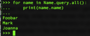
(Note that “Mark” appears on the main page since this record was added to the database as part of the fixture.)

Now, in your main app directory, you can run your tests by simply typing “pytest” in the command line. The result for our code here should look like this:

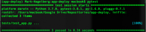
The three dots ‘…’ indicate that there were three tests and they each passed (if a test failed, one of these dots appear as an F).

Aside: during the creation of this post, I was puzzled to see that my code was running in the flask production environment, despite my configuration and environment variables clearly indicating that I was in development. Turns out there is another environment variable that needs to be set called FLASK_ENV, which defaults to “production”, turning off debug mode in Flask and throwing a warning when you run your application on the Flask development server.  To fix this, run `export FLASK_ENV=“development”` on the command line. Note that this must be set as an environment variable: adding it in config.py doesn’t work. I’ve updated this information in Part 2.  For further information in the Flask documentation, see here.

Resources

https://www.patricksoftwareblog.com/testing-a-flask-application-using-pytest/

https://piotr.banaszkiewicz.org/blog/2014/02/22/how-to-bite-flask-sqlalchemy-and-pytest-all-at-once/

It is good practice when developing a web application to set up different environments for deploying changes. The number and nature of environments that are used can vary, but we’ll be using the following commonplace architecture:

• Development Environment: Where you develop the web application, typically on your local machine.
• Testing Environment: Where you perform tests to help ensure the quality of your application.
• Staging Environment: Where you deploy the application for the purpose of conducting “integration tests” that testing the broader functionality of your web app.
• Production Environment: Where you deploy your web app to your users.

In this Part 2 of our web app deployment and maintenance project, we’ll begin to set up some of these environments, including a database with an extremely simple schema as well as some additions to our application to incorporate the database and configure the app.

To follow along, you can clone the repository:

git clone https://github.com/marknagelberg/app-deploy.git

And then go to the appropriate location in the code changes with the following command:

git checkout 75521eb0e3d

Finally, create the python environment with:

conda env create -f environment.yml

Installing Additional Python Packages

To start off, we’ll install a couple of additional packages to our app’s Conda environment:

• Flask-SQLAlchemy: SQLAlchemy is a fantastic Python library that provides a way of interacting with your database purely in python, without having to write SQL query strings. Another benefit of using SQLAlchemy and similar ORMs is the ability to easily swap out databases if you decide you want to change in the future. Flask-SQLAlchemy is an extension for Flask that makes it easier to incorporate SQLAlchemy into Flask apps.
• Flask-Migrate: A Flask extension that provides a lightweight wrapper around the Alembic database migration framework. This will come in handy later when we need to make changes to our database schema after it’s already been deployed to production.
• Flask-WTF: A Flask extension that makes it easy to work with web forms.
• psycopg2: An adapter for PostgreSQL databases in Python. PostgreSQL will be our database of choice and this package is required to connect it up to our application.

To install these applications, first start up the Conda environment with the following command:

source activate app-deploy

Then install the packages above with the following commands:

pip install Flask-SQLAlchemy

pip install flask-migrate

pip install Flask-WTF

conda install psycopg2

Installing and Setting Up the PostgreSQL Databases

Next, we need to install PostgreSQL. You can find the proper install for your system here.

Postgres comes with a handy front end terminal program called psql, which allows you to examine your database’s tables and records using SQL queries. We first use psql to initialize two of the databases we’ll be working with for our program: the development database and the test database.

First enter into psql by typing psql into the terminal:

From here, you can run a bunch of useful commands. For example \l lists all the databases you currently have in postgres:

For now, we’ll need to use psql to create two databases that we’ll call app_deploy_development and app_deploy_test. This is as simple as running the two commands below.

Running the command \l shows that these two databases have been created:

You can then exit postgres with the command \q or simply press control-d.

To be able to connect to this database from Flask / SQL Alchemy, we need the URL string associated with the database. In PostgreSQL, this takes the form:

postgresql://username:password@hostname:port/database

We’ll eventually be running the the development and test databases on localhost, so the hostname is ‘localhost’, the port is 5432 (this is a postgres default) and database is ’app_deploy_development’. You can confirm the port Postgres is running on by running the following command:

Configuring our Flask App

Now we’ll make some changes to the app so that the database is actually used.

FIrst we will begin to incorporate the application environments that we need. The main way to do this in Flask is through the configuration variables, which are stored in app.config variable (where app is the instance of your application).

The simplistic version of app.config is treated like a simple dictionary (e.g. you can set app.config[‘SECRET_KEY’] = ‘some_secret’), but this does not account for the fact that you need to work with different sets of configurations depending on how you’re running your application. Instead, a more flexible way to set up the app.config variable is to use a hierarchy of configuration classes, defined like this:

https://gist.github.com/marknagelberg/ccc001e4cf844bf9ddac6315029b339f

SQLALCHEMY_DATABASE_URI is an environmental variable required by SQLAlchemy to tell the extension where to find the database. Since these environmental variables are sensitive (they contain username and password information that you would not want to share), they are defined in your system’s environmental variables rather than including them in version control (you define these using the export command). Add the configuration code above is to a file called config.py in the app’s top directory.

Refactoring our App to use the Application Factory Pattern

We need to do some restructuring of our application to account for the database and implement the “application factory” pattern in Flask that allows us to provide different app instances with different configurations. We first move our app.py file into the /app folder. We also create an app/templates/ folder to store the front-end template that will hold the template for our front end form to enter names the and “hello world” message.

We also create /app/__init__.py:

https://gist.github.com/marknagelberg/e7d40c9b07c12db67033066e49392bec

This file stores our factory function ‘create_app’ that returns instances of the application. create_app takes a config_name argument, allowing us to create an app with the desired configuration option (e.g. create_app(‘development’), create_app(‘testing’), etc.) The configuration is assigned to the app within the factory function using the Flask app.config.from_object function along with the dictionary of configuration classes defined in config.py.

Adding the Database to our App

Rather than having just “Hello World”, we want to have our application make use of the database in some minimal way. So, we add a form where the user can enter names which are stored in the database inside a single table, consisting of a single column holding the names.

To define the database schema, we create a file called models.py:

https://gist.github.com/marknagelberg/8472a6e582dd07f14bae7d03bdd6b1ab

This file imports our database instance db. Here we define a ‘name’ string column, and an integer id that serves as a primary key (your table must have a primary key).

We also create a file create_app.py in the app’s top directory:

https://gist.github.com/marknagelberg/9bec1faf6673a94ed9ca1db163845ea7

This file is tasked with creating the instances of app from the create_app function defined in app/__init__.py. This function is what allows us to choose a particular configuration, which we define in an environment variable on our system called FLASK_CONFIG. It is also a place where we can do additional configuring of our newly generated application instance (e.g. creating commands for your app with the flask command line program by decorating functions with @app.cli.command()). This file may seem a little unnecessary now but it will come in handy later.

We also need to insert a form for the user to enter in data. We’ll use the assistance of the great Flask extension, Flask-WTF. With Flask-WTF, you define forms as classes that inherit from FlaskForm. Each of the class variables represents a field in the form that takes in certain types of values. Here our form is quite simple as it only takes a single field where the user can enter in names. There is also a ‘submit’ button which provides exactly what you expect.

https://gist.github.com/marknagelberg/eba3eb55421536c34a2649bfac05a213

Now that we have a form defined, we can define the new front end template index.html.

https://gist.github.com/marknagelberg/a00249c0c401bfe593a9500428beccaf

In our main application, we need to pass our NameForm class to render this template so we add the following code to app.py. Also note that, because of the way that we used the app_factory pattern, we must now use ‘BluePrints” for our view functions rather than defining routes in a single file directly to the app instance (blueprints are basically objects that can hold a bunch of an app’s routes and code and then can be registered with the application in the apps factory function).

https://gist.github.com/marknagelberg/a59dc1feb241dd02687be6b97d06fc1e

Running our Updated App With the Database

To run the application first define environmental variables:

• FLASK_APP, which tells the flask command line program where the flask application is located so that it can run it:

export FLASK_APP=create_app.py

• FLASK_CONFIG, which is the environmental variable that tells the program what environment your app should be running in. As a reminder, this value is used in create_app.py and references one of the values in the dict found in config.py.

export FLASK_CONFIG=development

• DEV_DATABASE_URL, which points to your development database. As a reminder, this is assigned to the environment variable SQLALCHEMY_DATABASE_URI in config.py.

export DEV_DATABASE_URL=”postgresql://<insert username>:<insert password>@localhost:5432/app_deploy_development”

Before you run the application the first time, you have to initialize the database. You only have to do this once, using the db.create_all() method provided by Flask-SQLAlchemy. From the top application directory run:

flask shell
>> from app import db
>> db.create_all()

Then you can exit the python interpreter with quit() or control-d.

Finally, run the application with:

flask run

Now, when you visit http://127.0.0.1:5000/, you should see this:

Your app should now be running with a live development database in the background ready to store whatever is entered into the form. To make sure it’s working, enter a few names into the form (for my test, I typed in “Foobar”, “Mark”, and “Joanna”). Then, in the terminal from the top directory in your app, write the command “flask shell” to run the python interpreter in the context of your app. This throws you into the python interpreter. We’ll then query the database to make sure our names exist:

Looks like we’re good to go! Just to be sure, I loop through the names to make sure they’re the values we expect:

In this series, I’m going to work through the process of deploying and maintaining a simple web application. The goal is for you to get an understanding of all the steps that may be involved in deploying a web app and maintaining it in production with modern tools and techniques.

To follow along in this series, it would help to have an understanding of the command line, python programming, and basic web application development. I’ll be using the Flask web development framework. You’re in my target audience if you’ve built simple Flask applications running locally, and you now want to deploy it and use related best practices, such as implementing development, staging, and production environments, using docker containers, and making changes to the application via continuous integration / continuous deployment (CI / CD) tools.

The focus here is not on the web application itself –  rather, it’s on the process of deployment and maintenance. I’m going to get into all the nuts and bolts related to getting the app running live and maintaining it in a smart way. Along the way, we’ll learn about the best practices around deploying a web application that I find are not readily available in many tutorials.

Table of contents:

Part 1 – Setting up the server (currently reading)
Part 2 – Setting up the Database and App Configuration
Part 3 – Adding Tests with Pytest
… To come, as I finish the series 🙂

Getting Started

As the basis for our adventure, we’ll start with the simplest Flask app possible: the hello world app from the Flask website.

To get the full code for this application, run:

git clone https://github.com/marknagelberg/app-deploy.git

You need install Conda, which is the tool I use for managing the python environments (see my related post here). The environment information is stored in environment.yml in the repository.

To create the python environment from the environment.yml file, run the following command in the main project directory (i.e. app-deploy/):

conda env create -f environment.yml

The conda environment is called ‘app-deploy’. To run the environment after you’ve created it, simply type (on Mac or Linux):

source activate app-deploy

Or on Windows:

activate app-deploy

For each part of this series, I will provide a git checkout command that will allow you to see the code in the state relevant to that part of the series.

To start off with the initial, most basic version of the application, run:

git checkout 75521eb0e3

The main document in the repository is a file called app.py that looks like this:

https://gist.github.com/marknagelberg/cb0084c0e4720a8dbc6d36b544909759

First activate the environment, which will add ‘(app-deploy)’ to your command line to indicate you are in the environment, like this:

Now that you are in the appropriate python environment, you can run:

python app.py

Which runs Flask’s development server and serves the app to http://127.0.0.1:5000/.

If you visit the site in the browser, you should see this:

Part 1 – Setting up the Server

As a first step in this process, we’re going to spin up a server that will ultimately run the web application in production.

An aside for data scientists: Running and configuring web servers is a valuable skill for data scientists. You often need to do this to run data-driven applications you build for others (you don’t want to be running these things on your desktop computer). Furthermore, there are many valuable tools and services out there for data scientists and their coworkers that are designed to run on a server, rather than as a desktop application (e.g. Apache Superset, which is a free and open source business intelligence dashboard like Tableau or PowerBI). Servers also come in handy for your own personal use even if you have no plans to deploy a web application. For example, your server can run scripts that automatically create reports and send you email notifications, or you can run web scrapers that collect data while you sleep.

Back in the day, you needed an on-site physical server to do this. Thankfully, modern cloud computing makes it incredibly easy and cheap to run your own server. There are a few good options out there, but in this series, I’m going to use a Digital Ocean “droplet”. 

First, create an account with Digital Ocean. Then, choose the option to create a droplet:

Then, choose the operating system that you want your server to run on. I went with Ubuntu, since it’s what I’m most familiar with. It has a large user base, and as a result, there is lots of online tutorials / documentation to help you troubleshoot when things go wrong.

Then choose the memory and CPU power of your server. I went with the smallest / cheapest one. It’s easy to “resize” your droplet later on if you realize you need more juice.

Now choose a datacenter region – this is the location where your server will run. I suggest picking a data center closest to you, or closest to where your users will be. For me, that’s their Toronto data center.

Finally, you have to specify an SSH key. This will allow you to use the ssh command line program to log into your server remotely (you’ll be working with your server entirely through the command line). DigitalOcean gives you the option to enter it right inside their online dashboard interface as a step in creating the droplet. They also provide this useful guide. Here’s what I did on my Mac.

1. Run the command:

ssh-keygen

This generates two files which represent the public-private key pairs that you’ll need to authenticate via SSH. Save these files in your ~/.ssh directory (this is the directory where the ssh program will automatically look when you attempt to log into the server). You’ll also get an option to add a password to the file, which is recommended as protection against your laptop being stolen and someone getting access to the files.

id_rsa and id_rsa.pub are the default names for these public / private key pairs. Since these already exist in my .ssh directory, I chose a different filename: app-deploy and app-deploy.pub.  

Once you create these files, you then need to copy the contents of the public key (i.e. the file ending in ‘.pub’) into the “New SSH Key” form that Digital Ocean provides when setting up your droplet:

After entering in your public key, you can click the button to create your server.

Finally, to login to my server I run:

ssh -i ~/.ssh/app_deploy root@server_ip_address

If you chose the default filename (id_rsa and id_rsa.pub), then you only need to run:

ssh root@server_ip_address

And congratulations – you are now logged into your own personal server running in the cloud!

It’s common wisdom among data scientists that 80% of your time is spent cleaning data, while 20% is the actual analysis.

There’s a similar issue when doing an empirical research study: typically, there’s tons of work to do up front before you get to the fun part (i.e. seeing and interpreting results).

One important up front activity in empirical research is figuring out the sample size you need. This is a crucial, since it significantly impacts the cost of your study and the reliability of your results. Collect too much sample: you’ve wasted money and time. Collect too little: your results may be useless.

Understanding the sample size you need depends on the statistical test you plan to use. If it’s a straightforward test, then finding the desired sample size can be just a matter of plugging numbers into an equation. However, it can be more involved, in which case a programming language like Python can make life easier. In this post, I’ll go through one of these more difficult cases.

Here’s the scenario: you are doing a study on a marketing effort that’s intended to increase the proportion of women entering your store (say, a change in signage). Suppose you want to know whether the change actually increased the proportion of women walking through. You’re planning on collecting the data before and after you change the signs and determine if there’s a difference. You’ll be using a two-proportion Z test for comparing the two proportions. You’re unsure how long you’ll need to collect the data to get reliable results – you first have to figure out how much sample you need!

Overview of the Two Proportion Z test

The first step in determining the required sample size is understanding the statical test you’ll be using. The two sample Z test for proportions determines whether a population proportion p₁ is equal to another population proportion p₂. In our example, p₁ and p₂ are the proportion of women entering the store before and after the marketing change (respectively), and we want to see whether there was a statistically significant increase in p₂ over p₁, i.e. p₂ > p₁.

The test test the null hypothesis: p₁ – p₂ = 0. The test statistic we use to test this null hypotheses is:

$latex Z = \frac{p_2 – p_1}{\sqrt{p*(1-p*)(\frac{1}{n_1} + \frac{1}{n_2})}}&s=4$

Where p* is the proportion of “successes” (i.e. women entering the store) in the two samples combined. I.e.

$latex p* = \frac{n_1p_1 + n_2p_2}{n_1 + n_2}&s=4$

Z is approximately normally distributed (i.e. ~N(0, 1)), so given a Z score for two proportions, you can look up its value against the normal distribution to see the likelihood of that value occurring by chance.

So how to figure out the sample size we need? It depends on a few factors:

• The confidence level: How confident do we need to be to ensure the results didn’t occur by chance? For a given difference in results, detecting it with higher confidence requires more sample. Typical choices here include 95% or 99% confidence, although these are just conventions.
• The percentage difference that we want to be able to detect: The smaller the differences you want to be able to detect, the more sample will be required.
• The absolute values of the probabilities you want to detect differences on: This is a little trickier and somewhat unique to the particular test we’re working with. It turns out that, for example, detecting a difference between 50% and 51% requires a different sample size than detecting a difference between 80% and 81%. In other words, the sample size required is a function of p₁, not just p₁ – p₂.
• The distribution of the data results: Say that you want to compare proportions within sub-groups (in our case, say you subdivide proportion of women by age group). This means that you need the sample to be big enough within each subgroup to get statistically significant comparisons. You often don’t know how the sample will pan out within each of these groups (it may be much harder to get sample for some). There are at least a couple of alternatives for you here: i) you could assume sample is distributed uniformly across subgroups ii) you can run a preliminary test (e.g. sit outside the store for half a day to get preliminary proportions of women entering for each age group).

So, how do you figure out sample sizes when there are so many factors at play? 

Figuring out Possibilities for Sample Sizes with Python

Ultimately, we want to make sure we’re able to calculate a difference between p₁ and p₂ when it exists. So, let’s assume you know that the “true” difference that exists between p₁ and p₂. Then, we can look at sample size requirements for various confidence levels and absolute levels of p₁.

We need a way of figuring out Z, so we can determine whether a given sample size provides statistically significant results, so let’s define a function that returns the Z value given p₁, p₂, n₁, and n₂.

[gist https://gist.github.com/marknagelberg/b6bfe3e2141f8eeaeb0f2537ccbed81f /]

Then, we can define a function that returns the sample required, given p₁ (the before probability), p_diff (i.e. p₂ – p₁), and alpha (which represents the p-value, or 1 minus the confidence level). For simplicity we’ll just assume that n₁ = n₂. If you know in advance that n₁ will have about a quarter of the size of n₂, then it’s trivial to incorporate this into the function. However, you typically don’t know this in advance and in our scenario an equal sample assumption seems reasonable.

The function is fairly simplistic: it counts up from n starting from 1, until n gets large enough where the probability of that statistic being that large (i.e. the p-value) is less than alpha (in this case, we would reject the null hypothesis that p₁ = p₂). The function uses the normal distribution available from the scipy library to calculate the p value and compare it to alpha. 

[gist https://gist.github.com/marknagelberg/42b3077db573bcce55e00f975b8e4fc5 /]

These functions we’ve defined provide the main tools we need to determine minimum sample levels required.

As mentioned earlier, one complication to deal with is the fact that the sample required to determine differences between p₁ and p₂ depend on the absolute level of p₁. So, the first question we want to answer is “what p₁ that would require the biggest sample size to determine a given difference with p₂?” Figuring this out allows you to calculate a lower bound on the sample you need for any p₁. If you calculate the sample for the p₁ with the highest required sample, you know it’ll be enough for any other p₁.

Let’s say we want to be able to calculate a 5% difference with 95% confidence level, and we need to find a p₁ that gives us the largest sample required. We first generate a list in Python of all the p₁ to look at, from 0% to 95% and then use the sample_required function for each difference to calculate the sample.

[gist https://gist.github.com/marknagelberg/6b0679187cd7ce110546e581417bf6c4 /]

Then, we plot the data with the following code.

[gist https://gist.github.com/marknagelberg/2ace5e06f7012c76936887d82eff6aaf /]

Which produces this plot:

This plot makes it clear that p₁ = 50% produces the highest sample sizes.

Using this information, let’s say we want to calculate the sample sizes required to calculate differences in p₁ and p₂ where p₂ – p₁ is between  2% and 10%, and confidence levels are 95% or 99%. To ensure we get a sample large enough, we know to set p₁ = 50%. We first write the code to build up the data frame to plot.

[gist https://gist.github.com/marknagelberg/4e647533f034a244ea3850e6ab5ec4da /]

Then we write the following code to plot the data with Seaborn.

[gist https://gist.github.com/marknagelberg/0c1845bf835da661851c948d837a0e95 /]

The final result is this plot:

This shows the minimum sample required to detect probability differences between 2% and 10%, for both 95% and 99% confidence levels. So, for example, detecting a difference of 2% at 95% confidence level requires a sample of ~3,500, which translates into n₁ = n₂ = 1,750. So, in our example, you would need about 1,750 people walking into the store before the marketing intervention, and 1,750 people after to detect a 2% difference in probabilities at a 95% confidence level.

Conclusion

The example shows how Python can be a very useful tool for performing “back of the envelope” calculations, such as estimates of required sample sizes for tests where this determination is not straightforward. These calculations can save you a lot of time and money, especially when you’re thinking about collecting your own data for a research project.

One of the best skills that you can develop is the ability to find talented people before anyone else does.

This great advice from Tyler Cowen (economist and blogger at Marginal Revolution) got me thinking: What are some strategies for finding talented but underrated people?

One possible source is Twitter. For a long time, I didn’t “get” Twitter, but after following Michael Nielsen’s advice I’m officially a convert. The key is carefully selecting the list of people you follow. If you do this well, your Twitter feed becomes a constant stream of valuable information and interesting people.

If you look carefully, you can find a lot of highly underrated people on Twitter, i.e. incredibly smart people that put out valuable and interesting content, but have a smaller following that you would expect.

These are the kinds of people that are the best to follow: you get access to insights that a lot of other people are not getting (since not many people are following them), and they are more likely to respond to queries or engage in discussion (since they have a smaller following to manage).

One option for finding these people is trial and error, but I wanted to see if it’s possible to quantify how underrated people are on Twitter and automate the process for finding good people to follow.

I call this the TURI (Twitter Underrated Index), because hey, it needs a name and acronyms make things sound so official.

Components of TURI

The index has three main components: Growth, Influence of Followers, and the Number of Followers.

Growth (G): The number of followers a user has per unit of content they have published (i.e. per tweet).

A user that is growing their Twitter following quickly suggests that they are underrated. It implies they are putting out quality content and people are starting to notice rapidly. The way I measure this is the number of followers a person acquires per Tweet.

Another possible measurement of growth is the number of followers the user has acquired per unit of time (i.e. number of followers divided by the length of time the Twitter account has existed). However, there are a couple of problems with this option:

• Twitter accounts can be dormant for years. For example, someone might start an account but not tweet for 5 years and then put out great content. Measuring growth in terms of time would unfairly punish these people.
• A person may have a strategy of Tweeting constantly. Some of the content results in followers, but the overall quality is still low. We are looking for people that publish great content, not necessarily people that put out a lot of content.

Influence of Followers (IF): The average number of the user’s follower’s followers.

In my opinion, the influence of a person’s following is the most important factor determining whether they are underrated on Twitter. Here’s a few reasons why:

• Influential people are, on average, better judges of good content.
• Influential people are more selective in who they decide to follow, especially if Twitter is an important part of their online “brand”.
• Influential people tend to engage with or are in some way related to other high quality people in their offline personal lives, and these people are more likely to appear in their Twitter feed even if they are not widely known or appreciated yet.

I’m somewhat biased toward this measure because, from my own personal experience, it has worked out really well when I browse through people who are followed by influential people on my feed. If I see someone followed by Tyler Cowen, Alex Tabarrok, Russ Roberts, Patrick Collison, and Marc Andreessen, and yet they only have 5,000 followers, then I’m pretty confident that person is currently underrated.

After some consideration, I believe the best way to measure the influence of a user’s followers with the data available in the Twitter API is taking the average number of the user’s follower’s followers.

I mulled over the possibility of using the median rather than the average, but decided against it: If someone with 1 million followers follows someone with 50 followers, I want to know more about that person, even though their TURI is high only because of that one highly influential follower. Outliers are good – we’re looking for diamonds in the rough.

Total Number of Followers (NF): The total number of followers the user currently has.

Our very definition of “underrated” in this context is when a user does not have as many followers as you expect, so total number of followers is obviously going to play an important role in TURI.

So to summarize the main idea behind TURI: if a person has a large number of “influential” followers, is growing their number of followers quickly relative to the volume of content they put out, and they still have a small number of total followers, then they are likely underrated.

Defining the Index

For any user i, we can calculate their Twitter Underrated Index (TURI) as:

$latex TURI_i = \frac{G_iIF_i}{NF_i}&s=4$

Where G is growth, IF is influence of followers, and NF is the number of followers.

This formula has the general relationships we are looking for: high growth in users for each unit of content, highly influential followers, and a low number of total followers all push TURI upward.

We can simplify the equation by rewriting G = NF / T, where T is the total number of tweets for the user. Cancelling out some terms, this gives us our final version of the index:

$latex TURI_i = \frac{IF_i}{T_i}&s=4$

In other words, our index of how under-rated a person is on twitter is given by the average number of i’s followers followers per tweet of user i.

Before calculating TURI for a group of users, there are a couple of pre-processing steps you will likely want to take to improve the results:

1. Filter out verified accounts. One of the shortcomings of TURI is that a user’s growth / trajectory (i.e. G) will be very high if they are already a celebrity. These people typically have a large number of followers per Tweet not because of the content they put out, but because they’ve attained fame already elsewhere. Luckily, Twitter has a feature called a “verified account”, which applies “if it is determined to be an account of public interest. Typically this includes accounts maintained by users in music, acting, fashion, government, politics, religion, journalism, media, sports, business, and other key interest areas”. This is a prime group to filter out, because we are not looking for well-known people.
2. Filter users by number of followers: There are a few reasons why you might want to only calculate TURI for users that have a following within some range (e.g. between 500 and 1,000):
   • Although there may be situations where a person with 500,000 followers is underrated, but this seems unlikely to be the kind of person you’re looking for so not worth the API resources.  
   • Filtering by some upper follower threshold mitigates the risk of including celebrities without verified accounts.
   • You limit the number of calls you make to the API. The most costly operation in terms of API calls is figuring out the influence of followers. The more followers a person has, the more API calls required to calculate TURI.

Trying out TURI

To test out the index, I calculated its value on a subset of 49 people that Tyler Cowen follows who have 1,000 or fewer followers (Tyler blogs at my favourite blog, inspired this project, and has good taste in people to follow).

The graph below illustrates TURI for these users (not including 4 accounts that were not accessible due to privacy settings). 

As you can see, one user (@xgabaix) is a significant outlier. Looking a bit more closely at the profile, this is Xavier Gabaix, a well known economist at Harvard University. His TURI is so high because he has several very influential followers and he has not tweeted yet. 

So did TURI fail here? I don’t think so, since this is very likely someone to follow if he was actually Tweeting. However, it does seem a little strange to put someone at the top of the list that doesn’t actually have any Twitter content.

So, I filtered again for users that have published at least 20 tweets:

The following chart looks solely at the various user’s IF (Influence of their Followers). Interestingly, another user @shanagement has the most influential followers by far. However, they rank in third place for overall TURI since they tweet significantly more than @davidbrooks13 or @davidhgillen.

Limitations

Of course, TURI has some shortcomings:

• Difficult to tell how well TURI works: The measures are based on intuition and there is obviously no “ground truth” data about how underrated twitter users actually are. So, we don’t really have a data-based method for seeing how well the index works and improving it systematically. For example, you might question is whether Growth G should be included in the index at all. I think there’s a good argument for it: if people get followers quickly per unit of content there must be something about that content that draws others. But, on the other hand, maybe they aren’t truly underrated. Maybe the truly underrated people have good content but your average Twitter user underestimates them even after reading a few posts. People don’t always know high quality when the see it.
• It takes a fairly long time to calculate TURI: This is due to Twitter rate limits of API requests. For example, calculating TURI for 49 Twitter users above took about an hour. It would take even longer for people with larger followings (remember, I only focused on people with 1,000 or fewer followers). So, if you want to do a large batch of people, it’s probably a good idea run this on a server on an ongoing basis and store user and TURI information into a database. 

Other ideas?

There are many many different ways you could potentially specify an index like this. Leave a comment or reach out to me on Twitter or email if you have any suggestions.

One other possible tweak is accounting for the number of people that the user follows. I notice that some Twitter users seem to have a strategy of following a huge number of people in the hopes of being followed back. In these cases, their following strategy may be the cause of their high growth and not the quality of their content. One solution is to adjust the TURI by multiplying by (Number of User’s Followers) / (Number of People the User Follows). This would penalize people that, for example, have 15,000 followers but follow 15,000 people themselves.

Technical Details

You can find the code I used to interact with the API and calculate TURI here. The code uses the python-twitter package, which provides a nice way of interacting with the Twitter API, abstracting away annoying details so you don’t have to deal with them (e.g. authenticating with OAuth, dealing with rate limits).

Dash is a tool designed for building interactive dashboards and web applications using only Python (no CSS, HTML, or JavaScript required). I came across Dash while surveying options for building dashboards and reporting tools in my current position as Data Scientist with the City of Winnipeg Transportation Division.

Why use Dash?

Some of the lowest-hanging fruit working as a data science involves simply getting the data in front of the right people in a way that is easily digestible and actionable. No fancy ML, just presenting data to the right people at the right time in the right format. Dashboards are often a great way of doing that.

However, they can be a pain to build. Off-the-shelf dashboard tools like Tableau and PowerBI can be expensive and limiting (you are constrained to the features that they choose to include in their software). Developing dashboards from scratch as a web application is also a pain, since that often requires writing CSS, HTML, and JavaScript: as a data scientist, your focus is typically programming in python or R and your job typically does not require being an expert in JavaScript.

Dash strikes a perfect middle ground for a data scientist, providing way more flexibility and customizability than off-the-shelf tools at a much lower cost (i.e. free), while still having an easy-to-use API that a python-oriented data scientist should not have difficulty grasping.

A Demo Dash app of Blog Post Data from Marginal Revolution

To become familiar with Dash and see what it can do, I started out with a simple dashboard using some of the the scraped blog post data from Marginal Revolution (see this post on the MR scraper project). You can find the dashboard here, which provides an interactive chart of the number of posts on Marginal Revolution over time for each author. You can choose any of the authors in the drop down box, and the relevant data shows up in the chart:

I have to say, I can’t believe how easy it was to build this dashboard. In total, it’s only 33 lines of python code (you can find the code here. It was also easy to deploy to heroku, following this guide.

How Dash Works

I highly recommend going through the Dash tutorial here, which walks you through app creation and the main components of Dash. Here I’ll give a high level overview of some key points.

Dash apps have two components: a layout component which describes how the application looks visually, and an interactivity component which specifies how your dashboard interacts with the user and responds to input.

Layout Component

The layout defines what the dashboard looks like. When defining the layout of your application, you create a hierarchical “tree” of components, and each component will come from one of the following two main classes:

• dash_html_components: This includes a component to represent every HTML tag. E.g. dash_html_components.H1(children = ‘Hello Dash’) adds <h1>Hello Dash</h1> to your dashboard.
• dash_core_components: This describes higher-level components that combine HTML, JavaScript, and CSS created through the React.js library. These components have an interactive element to them (e.g. graphs with tooltips). One of the key classes within dash_core_components is Graph. Graph components represent data visualizations created using plotly.js (Plotly is the company that created Dash). Graph provides 35 different chart types to meet your needs. Another nice feature included within dash_core_components is the ability to include Markdown, which is often more convenient for presenting text based copy in your dashboards. There are many other options available to you in the dash_core_components library to use in your dashboard (e.g. sliders, checkboxes, date ranges, interactive tables, tabs, and more – see the gallery here).

To define the layout for a page and the data contained within it, you nest these various components as appropriate. You assign this nested list to app.layout, where app = dash.Dash(). To see an example of how these components fit together and how they are rendered in the browser, see the getting started page on the Dash tutorial.

Interactivity Component

Another key feature of Dash is its ability to respond to user input and change the visualization accordingly (dashboards aren’t really of much use without this feature). Dash makes this functionality quite easy, although there is a bit too much to go into great detail in this blog post. Read part 2 of the Dash user guide.

In short, Dash lets you add interactivity by adding an @app.callback decorator to a Python function you write which takes the input from one of the layout components and returns outputs to send to another layout component that you want to change according to the new input.

You can have multiple inputs and multiple outputs. For example, if you want a graph that gives the user the option of filtering by multiple variables in your dataset, you can use multiple input filters. The function that you apply the @app.callback decorator to automatically fires whenever there are any changes to any of the inputs.

Deploying to Production

Dash uses the python Flask web application framework under the hood. Flask is an awesome, lightweight web application framework for Python that is definitely worth knowing (and relatively easy to learn given how stripped down it is). You can access the underlying Flask app instance using app.server where app is the instance of your dash app (i.e. app = Dash()).

Since the Dash app is essentially a Flask app under the hood, deploying a Dash app is the same as deploying a Flask app, and there are many guides online for deploying flask apps in a variety of situations. The Dash website provides some more details about deployment as well as steps for deploying to Heroku.

Comment below if you have any questions or if you want to share your experience using Dash!

Further Resources

Dash User Guide and Documentation
Plotly.py Documentation and Gallery
Dash Community Forum

Very often, data needs to be understood on a geographic basis. As a result, data scientists should be familiar with the main mapping tools at their disposal.

I have done quite a bit of mapping before, but given its central nature in my current position as a Transportation Assets Data Scientist with the City of Winnipeg, it quickly became clear that I need to do a careful survey of the geographic mapping landscape.

There is a dizzying array of options out there. Given my main programming language is python, I’ll start with tools in that ecosystem, but then I’ll move on to other software tools available for geographic analysis.

Mapping Tools in Python

GeoPandas

GeoPandas is a fantastic library that that makes munging geographic data in Python easy.

At its core, it is essentially pandas (a must-know library for any data scientist working with python). In fact, it is actually built on top of pandas, with data structures like “GeoSeries” and “GeoDataFrame” that extend the equivalent pandas data structures with useful geographic data crunching features. So, you get all the goodness of pandas, with geographic capabilities baked in.

GeoPandas works its magic by combining the capabilities of several existing geographic data analysis libraries that are each worth being familiar with. This includes shapely, fiona, and built in geographic mapping capabilities through descartes and matplotlib.

You can read spatial data into GeoPandas just like pandas, and GeoPandas works with the geographic data formats you would expect, such as GeoJSON and ESRI Shapefiles. Once you have the data loaded, you can easily change projections, conduct geometric manipulations, aggregate data geographically, merge data with spatial joins,  and conduct geocoding (which relies on the geocoding package geopy).

Basemap

Basemap is a geographic plotting library built on top of matplotlib, which is the granddaddy of python plotting libraries. Similarly to matplotlib, basemap is quite powerful and flexible, but at the cost of being somewhat time consuming and cumbersome to get the map you want.

Another notable issue is that Basemap recently came under new management in 2016 and is going to be replaced by Cartopy (described below). Although Basemap will be maintained until 2020, the Matplotlib website indicates that all development efforts are now focused on Cartopy and users should switch to Cartopy. So, if you’re planning on using Basemap, consider using…..

Cartopy

Cartopy provides geometric transformation capabilities as well as mapping capabilities. Similarly to Basemap, Cartopy exposes an interface to matplotlib to create maps on your data. You get a lot of mapping power and flexibility coming from matplotlib, but the downside is similar: creating a nice looking map tends to be relatively more involved compared to other options, with more code and tinkering required to get what you want.

geoplotlib

Geoplotlib is another geographic mapping option for Python that appears to be a highly flexible and powerful tool, allowing static map creation, as well as animated visualizations, and interactive maps. I have never used this library, and it appears to be relatively new, but it might be one to keep an eye out for in the future.

gmplot

gmplot allows you to easily plot polygons, lines, and points on google maps, using a “matplotlib-like interface”. This allows you to quickly and easily plot your data and piggy-back on the interactivity inherent to Google Maps. Plots available include polygons with fills, drop pins, scatter points, grid lines, and heatmaps. It appears to be a great option for quick and simple interactive maps. 

Mapnik

Mapnik is a toolkit written in C++ (with Python bindings) to produce serious mapping applications. It is aimed primarily at developing these mapping applications on the web. It appears to be a heavy duty tool that powers a lot of maps you see on the web today, including OpenStreetMap and MapBox.

Folium

Folium lets you tap into the popular leaflet.js framework for creating interactive maps, without having to write a single line of JavaScript. It’s a great library that I have used quite often in recent months (I used folium to generate all the visualizations for my Winnipeg tree data blog post).

Folium allows you to map points, lines, and polygons, produce choropleth maps and heat maps, create map layers (that users can enable or disable themselves), and produce pop-up tooltips for your geographic data (bonus: these tooltips support html so you can really customize them to make them look nice). There is also a good amount of customization possible with the markers and lines used on your map.

Overall, Folium strikes a great balance between features, customizability, and ease of programming.

Plotly

Plotly is a company offering a large suite of online data analytics and visualization tools. The focus of Plotly is providing frameworks that make it easier to present visualizations on the web. You write your code in Python (or R), talking to a plotly library and the visualizations are rendered using the extremely powerful D3.js library. For a taste of what is possible, check out their website, which showcases a bunch of mapping possibilities.

On top of the charts and mapping tools, they have a bunch of additional related products of interest on their website that are worth checking out. One that I’m particularly interested in is Dash, which allows you to create responsive data-driven web applications (mainly designed for dashboards) using only Python (no JavaScript or HTML required). This is something I’m definitely going to check out and will probably produce a “diving into data science” post in the near future.

Bokeh

Bokeh is a library specializing in interactive visualizations presented in the browser. This includes geographic data and maps. Similarly to Dash, there is also the possibility of using Bokeh to create interactive web applications that update data in real time and respond to user input (it does this with a “Bokeh Server”).

Other Tools for Mapping

There are obviously a huge amount of mapping tools outside of the python ecosystem. Here is a brief summary of a few that you might want to check out. Keep in mind that there are tons and tons of tools out there that are missing from this list. These are just some of the tools that I’m somewhat familiar with.

Kepler.gl

Kepler is a web-based application that allows you to explore geodata. It’s a brand spanking new tool released in late May 2018 by Uber. You can use the software live on its website – Kepler is a client side application with no server backend so all the data resides on your local machine / browser even.  It’s not just for use in on the Kepler website however; you can install the application and run it on localhost or a server, and you can also embed it into your existing web applications.

The program has some great features, with most of the basic features you would expect in an interactive mapping application, plus some really great bonus features such as split maps and playback. The examples displayed on the website are quite beautiful and the software is easy to use (accessible for use non-programmers).

This user guide provides more information on Kepler, what it can do, and how to do it. I’m very much looking forward to checking it out for some upcoming projects.

Mapbox

Mapbox provides a suite of tools related to mapping, aimed at developers to help you create applications that use maps and spatial analysis. It provides a range of services, from creating a nice map for your website to helping you build a geoprocessing application.

This overview provides a good idea of what’s possible. Mapbox provides a bunch of basemap layers, allow you to customize your maps, add your own data, and build web and mobile applications. It also provides options for extending functionality of web apps with tools like geocoding, directions, spatial analysis, and other features. Although Mapbox is not a free service, they do seem to have generous free API call limits (see their pricing here).

Heavy Duty GIS Applications

Not included here but also really important for people doing mapping are the full fledged GIS applications such as ArcGIS and QGIS. These are extremely powerful tools that are worth knowing as a geodata analyst. Note that ArcGIS is quite expensive; however, it is an industry standard so worth knowing. QGIS is also fairly commonly used and has the advantage of being free and open source.

Any glaring ommissions in this post? Let me know in the comments below or send me an email.

Further resources

Python data visualization libraries
Essential Python Geospatial Libraries
So You’d Like to Make a Map Using Python
Visualizing Geographic Data With Python
Geospatial Data with Open Source Tools in Python (YouTube) and accompanying GitHub Repo of Notebooks

Basemap

Basemap Tutorial
Map Making in Python with Basemap

Mapnik

Mapnik Wiki
Mapnik – Maybe the Best Python Mapping Platform Yet
Take Control of Your Maps

Folium

Python tutorial on making a multilayer Leaflet web map with Folium (YouTube)
Interactive Maps with Python (Three Parts)
Creating Interactive Crime Maps with Folium

Bokeh

Python: mapping data with python library Bokeh
Interactive Maps with Bokeh

In the Digging into Data Science Series, I dive into specific tools and technologies used in data science and provide a list of resources you can find to learn more yourself. I keep posts in this series updated on a regular basis as I learn more about the technology or find new resources. Post Last updated on May 28, 2018

If you’re familiar at all with Data Science, you have probably heard of Anaconda. Anaconda is a distribution of Python (and R) targeted towards people doing data science. It’s totally free, open-source, and runs on Windows, Linux, and Mac.

Up until recently, I basically treated my installation of Anaconda as a vanilla python install and was totally ignorant about the unique features and benefits it provides (big mistake). I decided to finally do some research into what Anaconda does and how to get the most out of it.

What is Anaconda and why should you use it?

Anaconda is much more than simply a distribution of Python. It provides two main features to make your life way easier as a data scientist: 1) pre-installed packages and 2) a package and environment manager called Conda.

Pre-installed packages

One of the main selling points of Anaconda is that is comes with over 250 popular data science packages pre-installed. This includes popular packages such as NumPy, SciPy, Pandas, Bokeh, Matplotlib, among many others. So, instead of installing python and running pip install a bunch of times for each of the packages you need, you can just install Anaconda and be fairly confident that  most what you’ll need for your project will be there.

Anaconda has also created an “R Essentials” bundle of packages for the R language as well, which is another reason to use Anaconda if you are an R programmer or expect to have to do some development in R.

In addition to the packages, it comes with other useful data science tools preinstalled:

• iPython / Jupyter notebooks: I’ll be doing a separate “Digging into Data Science Tools” post on this later, but Jupyter notebooks are an incredibly useful tool for exploring data in Python and sharing explorations with others (including non-Python programmers). You work in the notebook right in your web browser and can add python code, markdown, and inline images. When you’re ready to share, you can save your results to PDF or HTML.
• Spyder: Spyder is a powerful IDE for python. Although I personally don’t use it, I’ve heard it’s quite good, particularly for programmers who are used to working with tools like RStudio.

In addition to preventing you from having to do pip install a million times, having all this stuff pre-installed is also super useful you’re teaching a class or workshop where everyone needs to have the same environment. You can just have them all install Anaconda, and you’ll know exactly what tools they have available (no need to worry about what OS they’re running, no need to troubleshoot issues for each person’s particular system).

Package and environment management with Conda

Anaconda comes with an amazing open source package manager and environment manager called Conda.

Conda as a package manager

A package manager is a tool that helps you find packages, install packages, and manage dependencies across packages (i.e. packages often require certain other packages to be installed, and a package manager handles all this messiness for you).

Probably the most popular package manager for python is it’s built-in tool called pip. So, why would you want to use Conda over pip?

• Conda is really good at making sure you have the proper dependencies installed for data science packages. Researching for this blog post, I came across many stories of people having a horrible time installing important and widely used packages with pip (especially on Windows). The fundamental issue seems to be that many scientific packages in Python have external dependencies on libraries in other languages like C and pip does not always handle this well. Since Conda is a general-purpose package management system (i.e. not just a python package management system), it can easily install python packages that have external dependencies written in other languages (e.g. NumPy, SciPy, Matplotlib).
• There are many open source packages available to install through Conda which are not available through pip.
• You can use Conda to install and manage different versions of python (python itself is treated as just another package).
• You can still use pip while using Conda if you cannot find a package through Conda.

Together, Conda’s package management and along with the pre-installed packages makes Anaconda particularly attractive to newcomers to python, since it significantly lowers the amount of pain and struggle required to get stuff running (especially on Windows).

Conda as an environment manager

An “environment” is basically just a collection of packages along with the version of python you’re using. An environment manager is a tool that sets up particular environments you need for particular applications. Managing your environment avoids many headaches.

For example, suppose you have an application that’s working perfectly. Then, you update your packages and it no longer works because of some “breaking change” to one of the packages. With an environment manager, you set up your environment with particular versions of the packages and ensure that the packages are compatible with the application.

Environments also have huge benefits when sending your application to someone else to run (they are able to run the program with the same environment on their system) and deploying applications to production (the environment on your local development machine has to be the same as the production server running the application).

If you’re in the python world, you’re probably familiar with the built-in environment manager virtualenv. So why use Conda for environment management over virtualenv?

• Conda environments can manage different versions of python. In contrast, virtualenv must be associated with the specific version of python you’re running.
• Conda still gives you access to pip and pip packages are still tracked in Conda environments. 
• As mentioned earlier, Conda is better than pip at handling external dependencies of scientific computing packages.

For a great introduction on managing python environments and packages using Conda, see this awesome blog post by Gergely Szerovay. It explains why you need environments and basics of how to manage them in Conda. Environments can be a somewhat confusing topic, and like a lot of things in programming, there are some up-front costs in learning how to use them, but they will ultimately save tons of time and prevent many headaches.

Bonus: no admin privileges required

In Anaconda, installations and updates of packages are independent of system library or administrative privileges. For people working on their personal laptop, this may not seem like a big deal, but if you are working on a company machine where you don’t have access to admin privileges, this is crucial. Imagine having to run to IT whenever you wanted to install a new python package – It would be totally miserable and it’s not a problem to be underestimated.

Further resources / sources

• Conda Commands Cheat Sheet
• Conda Documentation
• Conda Quick Start Guide
• Conda: Myths and Misconceptions
• Does Conda replace the need for virtualenv? (Stack Overflow)
• Python Environment Management with Conda (includes description of using Anaconda alongside Jupyter Notebooks)
• Python Tutorial: Anaconda – Installation and Using Conda (YouTube)
• Table Comparison of conda vs. pip vs. virtualenv commands
• Understanding and using python virtualenvs from a Data Scientist perspective
• What advantages are there of using Anaconda? (Reddit)
• What is the difference between pyenv, virtualenv, anaconda? (Stack Overflow)
• Why should I use anaconda instead of traditional Python distributions for data science? (Quora)
• Why do we need Anaconda when we have pip? (Stack Overflow)
• Why you need Python environments and how to manage them with Conda